BioSANS - Symbolic and Numeric Software for Systems Biology

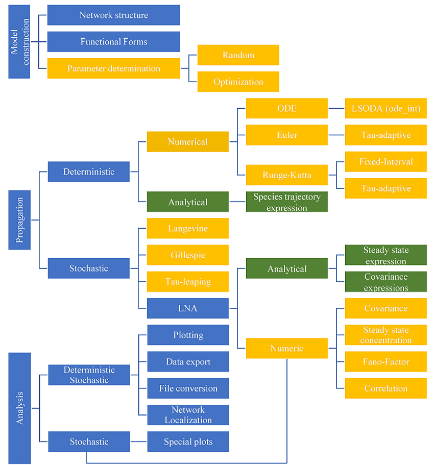
	BioSANS is a  free software for  systems biology  which is currently being developed in Academia Sinica Institute of Chemistry. The goal of this development is to make systems biology available to  non-domain experts in the easiest possible way. Currently,  BioSANS supports model creation, ODE propagation in both deterministic and stochastic settings, and post  simulation analysis. It can be used  either via the GUI, the  command line interface, and as a python import for experts users. BioSANS passed majority of the SBML semnatic and stochastic  test cases. It also  support parameter  estimation  and provides  an easy to  prepare input  which follows  basic  elementary equation  in chemistry. In the input  file, reaction, initial concentration,  and rate constants are required but the  propensity expression  is optional. The algorithm in BioSANS can infer the propensity from  the  reactions provided.  If the users need special  or non  mass  action  type propensity,  it can be encoded in the  topology file as well. Complicated conditional expression and concentration modification are also supported in the topology file.

	The following summarized the symbolic and numeric features currently supported;
	

	

Symbolic computation

1. Species analytical expression - works for most linear differential equation and few
   non-linear ordinary differential equations
2. LNA covariace matrix - works for most linear differential equation and few non-linear ODE
3. Steady state concentration - generally works for most problems especially linear ODE
4. Network localization - topology based sentitivity matrix

Numeric computation

1. Linear noise approximation
2. Parameter estimation
3. Network localization
4. Deterministic analysis (ODE integration)
  * odeint - python LSODA library
  * runge-kutta4 (tau-adaptive and fixed interval version)
  * Euler (two differnt types of tau-adaptive version)
5. Stochastic modeling
  * Chemical Langevine equation (tau-adaptive and fixed interval version)
  * Tau-leaping algorithm (2 different versions/implementation of Yang Cao's algorithm)
  * Gillespie direct method

Post-processing functions

1. Plotting (trajectory, density, etc.)
2. Calculation of correlation, covariance, fano-factor, etc.
3. Phase portrait
4. etc.

Graphical user interface

Console interface

Example commands:

propagate 
	A => B, 0.2 & 
	B => C, 0.3 
where 
	A=100 & 
	B=0.2 & 
	C=0 
using CLE 
with 
	tn=50 & 
	tlen=1000 & 
	miter=30 & 
	mult_proc=True & 
	fout=Traj1
;

It can also be type in the console in inline format as follows

propagate A => B, 0.2 & B => C, 0.3 where A=100 & B=0.2 & C=0 
using CLE with tn=50 & tlen=1000 & miter=2 & mult_proc=True & fout=Traj2;

BioSANS as a library import

from BioSANS2020 import biosans_lib as biosans

# Parameter estimation example


modelA = """
	Function_Definitions:
	Ao = 100
	Co = 0

	#REACTIONS
	A => B, -1
	B => C, -1

	@CONCENTRATION
	A, Ao
	B, -1
	C, Co
"""

dataA = """
	time,A,C
	0,100,0
	1,60.65306595,5.775043762
	2,36.78794412,17.97900716
	3,22.313016,31.82710907
	4,13.5335283,45.00173948
	5,8.208499842,56.53020973
	10,0.673794694,88.56392495
	15,0.055308438,97.30571352
	20,0.004539994,99.38712194
	25,0.000372665,99.86228791
	30,3.06E-05,99.96919344
	35,2.51E-06,99.99311965
	40,2.06E-07,99.99846425
	45.5,1.32E-08,99.99970501
	50,1.38E-09,99.99992352
"""

if __name__ == '__main__':
	my_model = biosans.model(modelA).data(dataA)
	data = my_model.run("k_est6")
	my_model.clean()